This is an example of an EDA carried out using R using an isolated environment created using renv

library(ggplot2)
library(dplyr)

Attaching package: 'dplyr'

The following objects are masked from 'package:stats':

    filter, lag

The following objects are masked from 'package:base':

    intersect, setdiff, setequal, union

library(palmerpenguins)
library(ggthemes)

df <- penguins[complete.cases(penguins),]
head(df)

# A tibble: 6 × 8
  species island    bill_length_mm bill_depth_mm flipper_length_mm body_mass_g
  <fct>   <fct>              <dbl>         <dbl>             <int>       <int>
1 Adelie  Torgersen           39.1          18.7               181        3750
2 Adelie  Torgersen           39.5          17.4               186        3800
3 Adelie  Torgersen           40.3          18                 195        3250
4 Adelie  Torgersen           36.7          19.3               193        3450
5 Adelie  Torgersen           39.3          20.6               190        3650
6 Adelie  Torgersen           38.9          17.8               181        3625
# ℹ 2 more variables: sex <fct>, year <int>

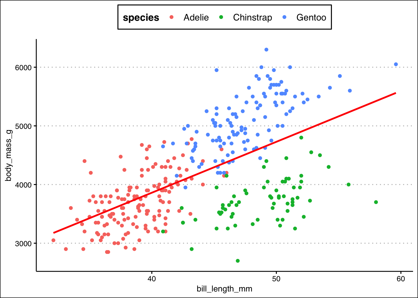
ggplot(df, aes(x = bill_length_mm, y = body_mass_g)) +
  geom_point(aes(color = species)) +
  geom_smooth(method = "lm", se = F, color = "red") +
  theme_clean() +
  theme(legend.position = "top")

`geom_smooth()` using formula = 'y ~ x'

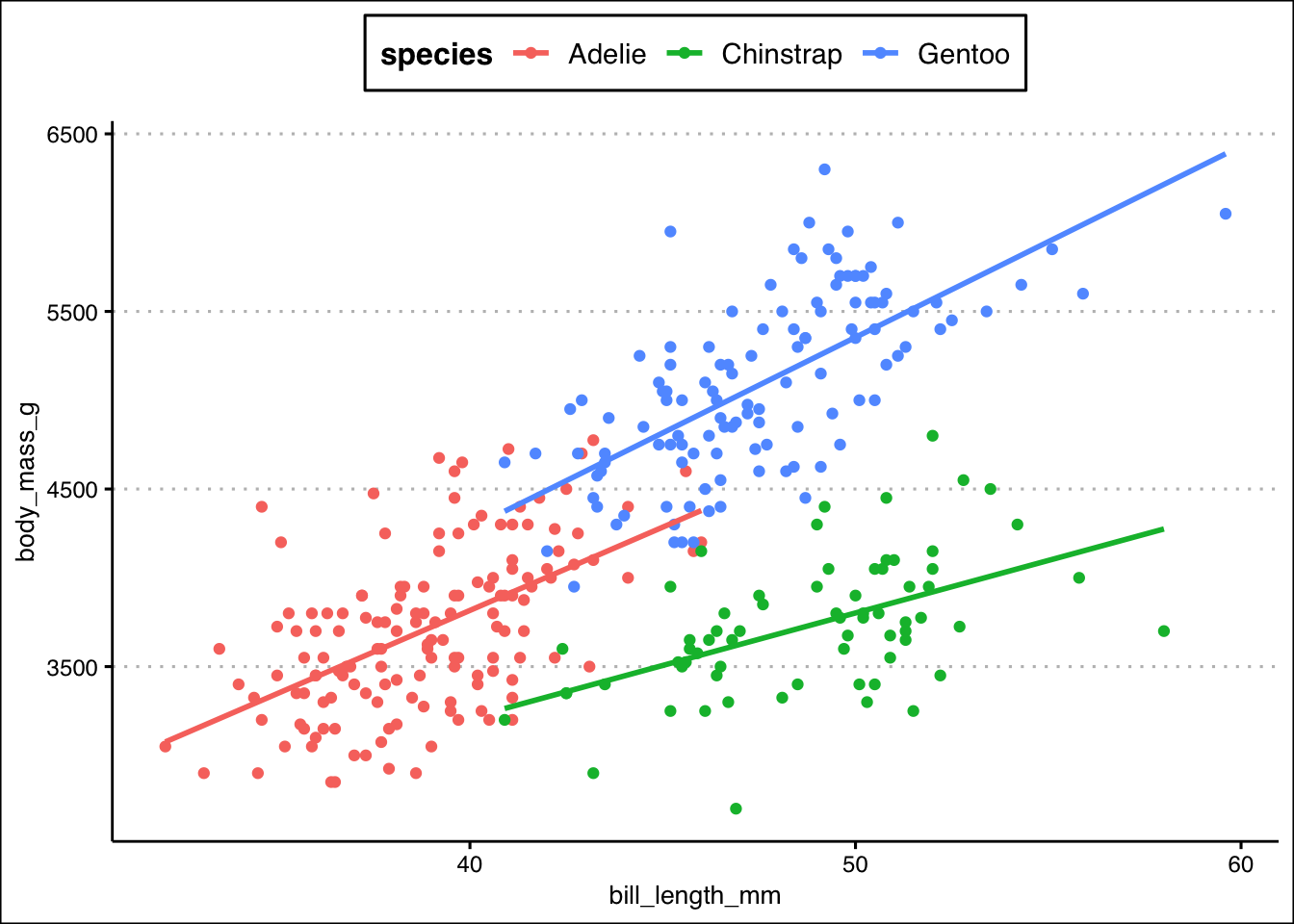
This shows a direct positive correlation between the two variables and some differences across species. In the modeling two methods are proposed. The first one is based off of a simple regression and shows an approximate fit to the data that is not very good (explains less than 40% of total variation in body mass). The second model employs a multiple linear regression with the categorical variable species to take into account the differences that might occur among the three different species in the sample. A graphical representation of this second model is given below.

ggplot(df, aes(x = bill_length_mm, y = body_mass_g, color = species)) +
  geom_point() +
  geom_smooth(method = "lm", se = F) +
  theme_clean() +
  theme(legend.position = "top")

`geom_smooth()` using formula = 'y ~ x'